Partitioning an Oracle table Tips

Partitioning is a divide-and-conquer approach to improving Oracle maintenance and SQL performance.  Anyone with un-partitioned databases over 500 gigabytes is courting disaster.  Databases become unmanageable, and serious problems occur: 

• Files recovery takes days, not minutes

• Rebuilding indexes (important to re-claim space and improve performance) can take days

• Queries with full-table scans take hours to complete

• Index range scans become inefficient

Preparing a new table partition is resource intensive and loading the new data into a staging area relieves and concurrent-user issues because the staging table is segregated from the ?live? data warehouse.

Please see related partitioning pages:

Justifying Oracle partitioning

Find latest partition in Oracle table

Oracle partitioning methods

oracle partitioning tips

Oracle Partitioning

Oracle interval partitioning tips

Oracle Partition Key Statistics & tuning

Once the data is loaded into the staging table, you can build the indexes, estimate the CBO statistics and use the ?exchange partition? command to load the table into the production environment with minimal impact.

Part 1: The Basics of Partitioning and How to Partition Tables.

Introduction

Oracle DBAs face an ever growing and demanding work environment. The only thing that may outpace the demands of the work place is the size of the databases themselves. Database size has grown to a point where they are now measured in the hundreds of gigabytes, and in some cases, several terabytes. The characteristics of very large databases (VLDB) demand a different style of administration. The administration of VLDB often includes the use of partitioning of tables and indexes.

Since partitioning is such an integral part of VLDB the remainder of this article will focus on how to partition, specifically, the partitioning of tables in an Oracle 9i Release 2 environment. Part 2 of this article will focus on the partitioning of indexes. The complete article will cover:

• Partitioning Defined
  
  

• When To Partition
  
  

• Different Methods Of Partitioning
  
  

• Partitioning Of Tables
  
  

• Partitioning Of Indexes

The organization of this article is modular so you can skip to a specific topic of interest. Each of the table partitioning methods (Range, Hash, List, Range-Hash and Range-List) will have its own section that includes code examples and check scripts.

Background

This article assumes that Oracle 9i Release 2 is properly installed and running. You will also need to have a user account that has a minimum of Create Table, Alter Table and Drop Table privileges. In addition to the basic privileges listed above, the creation of five small tablespaces (TS01, TS02, TS03, TS04, TS05) or changes to the tablespace clause will need to be done to use the examples provided in this article.

Ideally, you should try each of the scripts in this article under a DBA role. All scripts have been tested on Oracle 9i Release 2 (9.2) running on Windows 2000.

Partitioning Defined

The concept of divide and conquer has been around since the times of Sun Tzu (500 B.C.). Recognizing the wisdom of this concept, Oracle applied it to the management of large tables and indexes. Oracle has continued to evolve and refine its partitioning capabilities since its first implementation of range partitioning in Oracle 8. In Oracle 8i and 9i, Oracle has continued to add both functionality and new partitioning methods. The current version of Oracle 9i Release 2 continues this tradition by adding new functionality for list partitioning and the new range-list partitioning method.

When To Partition

There are two main reasons to use partitioning in a VLDB environment. These reasons are related to management and performance improvement.

Partitioning offers:

• Management at the individual partition level for data loads, index creation and rebuilding, and backup/recovery. This can result in less down time because only individual partitions being actively managed are unavailable.

• Increased query performance by selecting only from the relevant partitions. This weeding out process eliminates the partitions that do not contain the data needed by the query through a technique called partition pruning.

The decision about exactly when to use partitioning is rather subjective. Some general guidelines that Oracle and I suggest are listed below.

Use partitioning:

• When a table reaches a "large" size. Large being defined relative to your environment. Tables greater than 2GB should always be considered for partitioning.

• When performance benefits outweigh the additional management issues related to partitioning.

• When the archiving of data is on a schedule and is repetitive. For instance, data warehouses usually hold data for a specific amount of time (rolling window). Old data is then rolled off to be archived.

Take a moment and evaluate the criteria above to make sure that partitioning is advantageous for your environment. In larger environments partitioning is worth the time to investigate and implement.

Different Methods of Partitioning

Oracle 9i, Release 2 has five partitioning methods for tables. They are listed in the table below with a brief description.

For partitioning of indexes, there are global and local indexes. Global indexes provide greater flexibility by allowing indexes to be independent of the partition method used on the table. This allows for the global index to reference different partitions of a single table. Local indexes (while less flexible than global) are easier to manage. Local indexes are mapped to a specific partition. This one-to-one relationship between local index partitions and table partitions allows Oracle the ability to manage local indexes. Partitioning of indexes will be the focus of Part 2 of this article.

Detailed examples and code will be provided for each partitioning method in their respective sections. The use of the ENABLE ROW MOVEMENT clause is included in all of the examples of table partitioning to allow row movement if the partition key is updated.

Partitioning of Tables

Range Partitioning

Range partitioning was the first partitioning method supported by Oracle in Oracle 8. Range partitioning was probably the first partition method because data normally has some sort of logical range. For example, business transactions can be partitioned by various versions of date (start date, transaction date, close date, or date of payment). Range partitioning can also be performed on part numbers, serial numbers or any other ranges that can be discovered.

The example provided for range partition will be on a table named partition_by_range (what else would I call it?). The partition_by_range table holds records that contain the simple personnel data of FIRST_NAME, MIDDLE_INIT, LAST_NAME, BIRTH_MM, BIRTH_DD, and BIRTH_YYYY. The actual partitioning is on the following columns BIRTH_YYYY, BIRTH_MM, and BIRTH_DD. The complete DDL for the PARTITION_BY_RANGE table is provided in the script range_me.sql.

A brief explanation of the code follows. Each partition is assigned to its own tablespace. The last partition is the "catch all" partition. By using maxvalue the last partition will contain all the records with values over the second to last partition.

Hash Partitioning

Oracle's hash partitioning distributes data by applying a proprietary hashing algorithm to the partition key and then assigning the data to the appropriate partition. By using hash partitioning, DBAs can partition data that may not have any logical ranges. Also, DBAs do not have to know anything about the actual data itself. Oracle handles all of the distribution of data once the partition key is identified.

The hash_me.sql script is an example of a hash partition table. Please note that the data may not appear to be distributed evenly because of the limited number of inserts applied to the table.

A brief explanation of the code follows. The PARTITION BY HASH line is where the partition key is identified. In this example the partition key is AGE. Once the hashing algorithm is applied each record is distributed to a partition. Each partition is specifically assigned to its own tablespace.

List Partitioning

List partitioning was added as a partitioning method in Oracle 9i, Release 1. List partitioning allows for partitions to reflect real-world groupings (e.g.. business units and territory regions). List partitioning differs from range partition in that the groupings in list partitioning are not side-by-side or in a logical range. List partitioning gives the DBA the ability to group together seemingly unrelated data into a specific partition.

The list_me.sql script provides an example of a list partition table. Note the last partition with the DEFAULT value. This DEFAULT value is new in Oracle 9i, Release 2.

A brief explanation of the code follows. The PARTITION BY LIST line is where the partition key is identified. In this example, the partition key is STATE. Each partition is explicitly named, contains a specific grouping of VALUES and is contained in its own tablespace. The last partition with the DEFAULT is the "catch all" partition. This catch all partition should be queried periodically to make sure that proper data is being entered.

Composite Range-Hash Partitioning

Composite range-hash partitioning combines both the ease of range partitioning and the benefits of hashing for data placement, striping, and parallelism. Range-hash partitioning is slightly harder to implement. But, with the example provided and a detailed explanation of the code one can easily learn how to use this powerful partitioning method.

The range_hash_me.sql script provides an example of a composite range-hash partition table.

A brief explanation of the code follows. The PARTITION BY RANGE clause is where we shall begin. The partition key is (BIRTH_YYYY, BIRTH_MM, BIRTH_DD) for the partition. Next, the SUBPARTITION BY HASH clause indicates what the partition key is for the subpartition (in this case FIRST_NAME, MIDDLE_INIT, LAST_NAME). A SUBPARTITION TEMPLATE then defines the subpartition names and their respective tablespace. Subpartitions are automatically named by Oracle by concatenating the partition name, an underscore, and the subpartition name from the template. Remember that the total length of the subpartition name should not be longer than thirty characters including the underscore.

I suggest that, when you actually try to build a range-hash partition table, you do it in the following steps:

• Determine the partition key for the range.

• Design a range partition table.

• Determine the partition key for the hash.

• Create the SUBPARTITION BY HASH clause.

• Create the SUBPARTITION TEMPLATE.

Do Steps 1 and 2 first. Then you can insert the code created in Steps 3 -5 in the range partition table syntax.

Composite Range-List Partitioning

Composite range-list partitioning combines both the ease of range partitioning and the benefits of list partitioning at the subpartition level. Like range-hash partitioning, range-list partitioning needs to be carefully designed. The time used to properly design a range-list partition table pays off during the actual creation of the table.

The range_list_me.sql script provides an example of a composite range-list partition table.

A brief explanation of the code follows. The PARTITION BY RANGE clause identifies the partition key (BIRTH_YYYY, BIRTH_MM, BIRTH_DD). A SUBPARTITION TEMPLATE then defines the subpartition names and their respective tablespace. Subpartitions are automatically named by Oracle by concatenating the partition name, an underscore, and the subpartition name from the template. Remember that the total length of the subpartition name should not be longer than thirty characters including the underscore.

When building a range-list partition table you may want to refer to the steps mentioned at the end of the Composite Range-List section. The only difference is in Step 4. Instead of "Create the SUBPARTITION BY HASH clause" it would read, "Create the SUBPARTITION BY LIST clause" for the range-list partition table.

Part 2: Partitioning of Indexes

In Part 1 of "Partitioning in Oracle 9i Release 2," we learned how to use the various table partitioning methods in the latest release of Oracle. We will now continue on and learn about Globally Partitioned and Locally Partitioned Indexes. We will cover:

• Background/Overview

• Globally Partitioned Indexes

• Locally Partitioned Indexes

• When To Use Which Partitioning Method

• Real-Life Example

Background

This article assumes that Oracle 9i Release 2 is properly installed and running. You will also need to have a user account that has a minimum of Create Index, Alter Index and Drop Index privileges. In addition to the basic privileges listed above, the creation of five small tablespaces (ITS01, ITS02, ITS03, ITS04, ITS05) or changes to the tablespace clause will need to be done to use the examples provided in this article.

Ideally, you should try each of the scripts in this article under a DBA role. All scripts have been tested on Oracle 9i Release 2 (9.2) running on Windows 2000. The examples below build off of the examples that were used in Part 1 of this article.

Globally Partitioned Indexes

There are two types of global indexes, non-partitioned and partitioned. Global non-partitioned indexes are those that are commonly used in OLTP databases (refer to Figure1). The syntax for a globally non-partitioned index is the exactly same syntax used for a "regular" index on a non-partitioned table. Refer to gnpi_me.sql (http://www.dbazine.com/code/GNPI_ME.SQL) for an example of a global non-partitioned index.

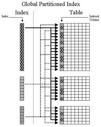
The other type of global index is the one that is partitioned. Globally partitioned indexes at this time can only be ranged partitioned and has similar syntactical structure to that of a range-partitioned table. gpi_me.sql (http://www.dbazine.com/code/GPI_ME.SQL) is provides for an example of a globally partitioned index. Note that a globally partitioned index can be applied to any type of partitioned table. Each partition of the globally partitioned index can and may refer to one or more partitions at the table level. For a visual representation of a global partitioned index refer to Figure 2.

The maintenance on globally partitioned indexes is a little bit more involved compared to the maintenance on locally partitioned indexes. Global indexes need to be rebuilt when there is DDL activity on the underlying table. The reason why they must be rebuilt is that DDL activity often causes the global indexes to be usually marked as UNUSABLE. To correct this problem there are two options to choose from:

• Use ALTER INDEX <index_name> REBUILD; or

• Use UPDATE GLOBAL INDEX clause when using ALTER TABLE.

The syntax for the ALTER INDEX statement is relatively straightforward so we will only focus on the UPDATE GLOBAL INDEX clause of the ALTER TABLE statement. The UPDATE GLOBAL INDEX is between the partition specification and the parallel clause. The partition specification can be any of the following:

• ADD PARTITION | SUBPARTITION (hash only)

• COALESCE PARTITION | SUBPARTITION

• DROP PARTITION

• EXCHANGE PARTITION | SUBPARTITION

• MERGE PARTITION

• MOVE PARTITION | SUBPARTITION

• SPLIT PARTITION

• TRUNCATE PARTITION | SUBPARTITION

For example:

ALTER TABLE <TABLE_NAME>
<PARTITION SPECIFICATION>
UPDATE GLOBAL INDEX
PARALLEL (DEGREE #)

Locally Partitioned Indexes

Locally partitioned indexes are for the most part very straightforward. The lpi_me.sql (http://www.dbazine.com/code/LPI_ME.SQL) script shows examples of this type of index. In the script, locally partitioned indexes are created on three differently partitioned tables (range, hash, and list). Figure 3 gives a visual representation of how a locally partitioned index works.

Extra time should be allocated when creating locally partitioned indexes on range-hash or range-list partitioned tables. There are a couple reasons that extra time is needed for this type of index. One of the reasons is a decision needs to be made on what the index will be referencing in regards to a range-hash or range-list partitioned tables. A locally partitioned index can be created to point to either partition level or subpartition level.

Script lpi4cpt1_me.sql (http://www.dbazine.com/code/LPI4CPT1_ME.SQL) is the example for the creation of two locally partitioned indexes. This scripts show how to create a locally partitioned index on both a range-hash and range-list partitioned tables at the partition level. Each of the partitions of the locally partitioned indexes is assigned to its own tablespace for improved performance.

When creating a locally partitioned index one needs to keep in mind the number of subpartitions of the range-hash or range-list partitioned table being indexed. Reason being, is that the locally partitioned index will need to reference each subpartition of the range-hash or range-list partitioned table. So, for the locally partitioned index created by lpi4cpt2.me.sql , this means that one index references twenty-five different subpartitions. For a visual representation of this refer to Figure 4. Script is provided as an example of locally partitioned index on a range-list partition table.

Note: At this time Oracle has not implemented a SUBPARTITION TEMPLATE clause for the creation of locally partitioned indexes on range-hash or range-list partition tables. This means that you need to type everything out as in the examples in lpi4cpt2_me.sql and lpi4cpt3_me.sql.

Maintenance of locally partitioned indexes is much easier than the maintenance of globally partitioned indexes. Whenever there is DDL activity on the underlying indexed table Oracle rebuilds the locally partitioned index.

This automatic rebuilding of locally partitioned indexes is one reason why most DBAs prefer locally partitioned indexes.

When to Use Which Partitioning Method

There are five different table partitioning methods (range, hash, list, range-hash and range-list) and three for indexes (global non-partitioned, global partitioned and locally partitioned). So, the obvious question is: "When do I use which combination of table and index partitioning?" There is no concrete answer for that question. However, here are some general guidelines on mixing and matching table and index partitioning.

• First determine if you need to partition the table.
  • Refer to Part 1 of this article under "When To Partition"

• Next decide which table partitioning method is right for your situation.
  • Each method is described in Part 1 of this article under "Different Methods of Partitioning"

• Determine how volatile the data is.
  • How often are there inserts, updates and deletes?

• Choose your indexing strategy: global or local partitioned indexes.
  • Each type has its own maintenance consideration.

These guidelines are good place to start when developing a partitioning solution.

Real Life Example

The "rolling window" concept of only retaining a certain amount of data is the norm in most data warehousing environments. This rolling window can also used to archive data from an OLTP system. For our example we will assume that there is a twelve month rolling window.

Our example will cover the following steps:

• Create a range partition table that has a locally partitioned index.

• Use "CREATE TABLE . . AS" to copy the data into a separate table.

• Archive off the table created to hold the rolled off data.

• Drop last month partition.

• Add new months partition.

Script example.sql is an annotated code of the example above.

Part 3: Partitioning in Oracle 10g and Oracle 11g

New in Oracle 10g

Each version release of Oracle comes with its own exciting set of new features. The following is a list of some partitioning features for Oracle 10g:

Improvements for VLDB such as data warehouses. These users depend on partitioned tables.

• Maximum number of partitions per object: This has been increased from 64K-1 to 1024K-1. This increase in the maximum number of partitions allowed creates much higher flexibility with regard to granularity of partitioned objects as well as creating many more partitioning approaches for each user to consider.

• Enhanced Dynamic Partition Pruning: For VLDB's, this feature enhances partition pruning for complex queries. For some, this can provide enhanced performance for a more robust set of complex queries.

• Resource Optimized DROP TABLE for Partitioned Tables: When using PURGE mode to drop large partitioned tables, the result is a large number of partions that have to be removed from the system logically. During the DROP operation, the large partitioned table is internally split to drop chunks of partitions. This new feature gives the capability of transparently dropping such an object in an incremental fashion. This can help with run-times and help optimize resource consumption.

• Partition Change Tracking Refresh Without Materialized View Logs: With this feature, Partition Change Tracking Refresh (PCT) does not require materialized view logs. Combining PCT with a fast refresh enables a refresh where one table is using PCT and the other is using materialized view logs. This can be a faster refresh, and now materialized views can be used without the overhead of materialized view logs.

Not just VLDBs benefitted with the release of Oracle 10g. Partionining on indexes also got a hand up:

• Online Indexing for Local Partitioned Index: This feature allows online indexing for local partitioned indexes. This means it is now possible to create an index on a partition while updating it. This also holds true with with unpartitioned indexes.

• Fast Partition Split for Partitioned Index Organized Tables: This feature enhances the SPLIT command. Historically, the SPLIT command moved each of the rows from an existing partition into one of the two new partitions following the split of a single partition of an index organized table into two new partitions. The performance enhancement here is that rows do not have to be moved if all of the rows in the existing partition fall into one of the new partitions.

It is possible to ADD, MERGE and SPLIT table partitions in a version-enabled table through the use of the alter_option parameter with the AlterVersionedTable procedure.

New in Oracle 11g

• REF partitioning: The 11g REF partitioning allows you to partition a table based on the values of columns within other tables. Source: Mark Rittman

• Partitioning: Partitioning by logical object and automated partition creation.

• New Oracle11g Advisors - New 11g Oracle Streams Performance Advisor and Partitioning Advisor. Source: Mark Rittman

• Interval Partitioning - Robert Freeman notes that 11g "interval Partitioning makes it easier to manage partitions":

"Wouldn't it be nice if you could just tell Oracle you wanted to partition every month and it would create the partitions for you? That is exactly what interval partitioning does."

"This is a new 11g partitioning scheme that automatically creates time-based partitions as new data is added." Source: Mark Rittman

"This is a marvelous one ! You can now partition by date, one partition per month for example, with automatic partition creation." Source: Laurent Schneider

Here is an example:

create table selling_stuff_daily
( prod_id number not null, cust_id number not null
, sale_dt date not null, qty_sold number(3) not null
, unit_sale_pr number(10,2) not null
, total_sale_pr number(10,2) not null
, total_disc number(10,2) not null)
partition by range (sale_dt)
interval (numtoyminterval(1,'MONTH'))
( partition p_before_1_jan_2007 values
less than (to_date('01-01-2007','dd-mm-yyyy')));

Note the interval keyword. This defines the interval that you want each partition to represent. In this case, Oracle will create the next partition for dates less than 02-01-2007 when the first record that belongs in that partition is created."

• Improved SQL Access Advisor - The 11g SQL Access Advisor gives partitioning advice, including advice on the new interval partitioning. Interval partitioning is an automated version of range partitioning, where new equally-sized partitions are automatically created when needed. Both range and interval partitions can exist for a single table, and range partitioned tables can be converted to interval partitioned tables.