 |
|
Oracle full table scan tips
Oracle Tips by Burleson Consulting |
This is an excerpt from my latest book "Oracle
Tuning: The Definitive Reference". It’s critical to understand that a full-table scan is a symptom of
a possible sub-optimal SQL plan. While not all full scans are
evil to performance, full table scans are a symptom of other common
tuning problems like missing indexes and sub-optimal schema statistics
(dbms_stats).
Remember, for small tables, a full-table scan is better than a
full-scan, but a large-table full-table scan should always be examined
as a “possible” problem.
Full scan I/O is cheaper than index
I/O
When Oracle reads a table front to back in
a full-table scan, we
save a great deal of disk latency. Remember, 95% of the disk
latency is the time required for the read-write head to move itself
under the proper cylinder. Once there, the read-write head sits
idle and the platter spins beneath it, and Oracle can read-in data
blocks as fast as the disk platter can spin, a processed called the
“db file scattered read”.
Oracle data files that are
using Automatic Storage Management (ASM) have implemented the SAME
principle (stripe and mirror everywhere), a RAID-10 combination of
disk striping and mirroring. Even though a data file is striped
across many disk spindles, it’s the “stripe size” that mandates how
many adjacent data block reside on disk, and the average latency for
full-scan I/O will be noticeably faster than index access, which
Oracle calls “db file sequential read” operations.
When a large-table full-table scan is evil
While we see that full-table scans are not evil, they do indeed
signal a “possible” tuning opportunity. Unnecessary large table
full-table scans can cause a huge amount of unnecessary I/O, placing a
processing burden on the entire database.
But how to we tell
when a large-table full-table scan is evil? One measure is to
compare the number of data block touches (consistent_gets) with the
number of rows returned by the SQL.
Whenever a SQL has a small
number of rows are returned, you can compare the number of rows in the
table to the number of rows returned to get a general idea of the
efficiency of a query. Anytime that you see a large-table
full-table scan that fetches less than 20% of the rows in the table,
you should investigate further to see if the full-scan is legitimate,
or whether you have a missing index.
Note:
These scripts
below will only track SQL that you have directed Oracle to capture via your
top SQL settings in AWR or STATSPACK, and STATSPACK and AWR will not
collect "transient SQL" that did not appear in v$sql at snapshot time.
Hence, not all SQL will
appear in these reports. See my notes here on
adjusting the SQL capture thresholds and
What SQL is
included in AWR/STATSPACK tables?
Tracking full scan access with AWR
All of the specific SQL access methods can be counted and their
behavior tracked over time. This is especially important for
large-table full-table scans (LTFTS) because they are a common
symptom of suboptimal execution plans (i.e. missing indexes).
Once it has been determined that the large-table full-table scans
are legitimate, the DBA must know those times when they are executed
so that a selective parallel query can be implemented, depending on
the existing CPU consumption on the server. OPQ drives up CPU
consumption, and should be invoked when the server can handle the
additional load.
Also see this script for
counting Oracle full table scans using v$sql_plan.
ttile ‘Large Full-table scans|Per Snapshot Period’
col c1 heading ‘Begin|Interval|time’ format a20
col c4 heading ‘Full table scan|Count’ format 999,999
break on c1 skip 2
break on c2 skip 2
select
to_char(sn.begin_interval_time,'yy-mm-dd hh24') c1,
count(1) c4
from
dba_hist_sql_plan p,
dba_hist_sqlstat s,
dba_hist_snapshot sn,
dba_segments o
where
SEE CODE DEPOT FOR FULL SCRIPTS
p.object_owner <> 'SYS'
and
p.object_owner = o.owner
and
p.object_name = o.segment_name
and
o.blocks > 1000
and
p.operation like '%TABLE ACCESS%'
and
p.options like '%FULL%'
and
p.sql_id = s.sql_id
and
s.snap_id = sn.snap_id
group by
to_char(sn.begin_interval_time,'yy-mm-dd hh24')
order by
1;
The output below shows the overall total counts for tables that
experience large-table full-table scans because the scans may be due
to a missing index.
Large Full-table scans
Per Snapshot Period
Begin
Interval FTS
time Count
-------------------- --------
04-10-18 11 4
04-10-21 17 1
04-10-21 23 2
04-10-22 15 2
04-10-22 16 2
04-10-22 23 2
04-10-24 00 2
This data can be easily plotted to see the trend for a database as
shown in Figure 15.25:
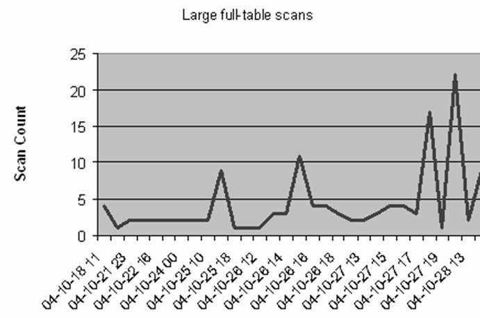
Figure 15.25:
– Trends of large-table
full-table scans
__________________________________________________
|

|
One of the most common manifestations of suboptimal SQL
execution is a large-table full-table scan.
Whenever an
index is missing, With a full-table scan, Oracle may be forced to read every row in
the table when an index might be faster. |
__________________________________________________
If the large-table full-table scans are legitimate, the DBA will
want to know the periods that they are invoked, so Oracle Parallel
Query (OPQ) can be invoked to speed up
the scans as shown in the
awr_sql_access_hr.sql script that follows:
ttile ‘Large Tabe Full-table scans|Averages per Hour’
col c1 heading ‘Day|Hour’ format a20
col c2 heading ‘Full table scan|Count’ format 999,999
break on c1 skip 2
break on c2 skip 2
select
to_char(sn.begin_interval_time,'hh24') c1,
count(1) c2
from
dba_hist_sql_plan p,
dba_hist_sqlstat s,
dba_hist_snapshot sn,
dba_segments o
where
SEE CODE DEPOT FOR FULL SCRIPTS
p.object_owner <> 'SYS'
and
p.object_owner = o.owner
and
p.object_name = o.segment_name
and
o.blocks > 1000
and
p.operation like '%TABLE ACCESS%'
and
p.options like '%FULL%'
and
p.sql_id = s.sql_id
and
s.snap_id = sn.snap_id
group by
to_char(sn.begin_interval_time,'hh24')
order by
1;
The following output shows the average number of large-table
full-table scans per hour.
Large Table Full-table scans
Averages per Hour
Day FTS
Hour Count
-------------------- --------
00 4
10 2
11 4
12 23
13 16
14 6
15 17
16 10
17 17
18 21
19 1
23 6
The script below shows the same data for day of the week:
ttile ‘Large Table Full-table scans|Averages per Week Day’
col c1 heading ‘Week|Day’ format a20
col c2 heading ‘Full table scan|Count’ format 999,999
break on c1 skip 2
break on c2 skip 2
select
to_char(sn.begin_interval_time,'day') c1,
count(1) c2
from
dba_hist_sql_plan p,
dba_hist_sqlstat s,
dba_hist_snapshot sn,
dba_segments o
where
SEE CODE DEPOT FOR FULL SCRIPTS
p.object_owner <> 'SYS'
and
p.object_owner = o.owner
and
p.object_name = o.segment_name
and
o.blocks > 1000
and
p.operation like '%TABLE ACCESS%'
and
p.options like '%FULL%'
and
p.sql_id = s.sql_id
and
s.snap_id = sn.snap_id
group by
to_char(sn.begin_interval_time,'day')
order by
1;
The following sample query output shows specific times the database
experienced large table scans.
Large Table Full-table scans
Averages per Week Day
Week FTS
Day Count
-------------------- --------
sunday 2
monday 19
tuesday 31
wednesday 34
thursday 27
friday 15
Saturday 2
The awr_sql_scan_sums.sql
script will show the access patterns of usage over time. If a DBA
is really driven to know their system, all they need to do is
understand how SQL accesses the tables and indexes in the database
to provide amazing insight. The optimal instance configuration for
large-table full-table scans is quite different than the
configuration for an OLTP databases, and the report generated by the
awr_sql_scan_sums.sql
script will quickly identify changes in table access patterns.
col c1 heading ‘Begin|Interval|Time’ format a20
col c2 heading ‘Large|Table|Full Table Scans’ format 999,999
col c3 heading ‘Small|Table|Full Table Scans’ format 999,999
col c4 heading ‘Total|Index|Scans’ format 999,999
select
f.c1 c1,
f.c2 c2,
s.c2 c3,
i.c2 c4
from
(
select
to_char(sn.begin_interval_time,'yy-mm-dd hh24') c1,
count(1) c2
from
dba_hist_sql_plan p,
dba_hist_sqlstat s,
dba_hist_snapshot sn,
dba_segments o
where
SEE CODE DEPOT FOR FULL SCRIPTS
p.object_owner <> 'SYS'
and
p.object_owner = o.owner
and
p.object_name = o.segment_name
and
o.blocks > 1000
and
p.operation like '%TABLE ACCESS%'
and
p.options like '%FULL%'
and
p.sql_id = s.sql_id
and
s.snap_id = sn.snap_id
group by
to_char(sn.begin_interval_time,'yy-mm-dd hh24')
order by
1 ) f,
(
select
to_char(sn.begin_interval_time,'yy-mm-dd hh24') c1,
count(1) c2
from
dba_hist_sql_plan p,
dba_hist_sqlstat s,
dba_hist_snapshot sn,
dba_segments o
where
p.object_owner <> 'SYS'
and
p.object_owner = o.owner
and
p.object_name = o.segment_name
and
o.blocks < 1000
and
p.operation like '%INDEX%'
and
p.sql_id = s.sql_id
and
s.snap_id = sn.snap_id
group by
to_char(sn.begin_interval_time,'yy-mm-dd hh24')
order by
1 ) s,
(
select
to_char(sn.begin_interval_time,'yy-mm-dd hh24') c1,
count(1) c2
from
dba_hist_sql_plan p,
dba_hist_sqlstat s,
dba_hist_snapshot sn
where
SEE CODE DEPOT FOR FULL SCRIPTS
The sample output looks like the following, where there is a
comparison of index versus table scan access. This is a very
important signature for any database because it shows, at a glance,
the balance between index (OLTP) and data warehouse type access.
Large Small
Begin Table Table Total
Interval Full Table Full Table Index
Time Scans Scans Scans
-------------------- ---------- ---------- --------
04-10-22 15 2 19 21
04-10-22 16 1 1
04-10-25 10 18 20
04-10-25 17 9 15 17
04-10-25 18 1 19 22
04-10-25 21 19 24
04-10-26 12 23 28
04-10-26 13 3 17 19
04-10-26 14 18 19
04-10-26 15 11 4 7
04-10-26 16 4 18 18
04-10-26 17 17 19
04-10-26 18 3 17 17
04-10-27 13 2 17 19
04-10-27 14 3 17 19
04-10-27 15 4 17 18
04-10-27 16 17 17
04-10-27 17 3 17 20
04-10-27 18 17 20 22
04-10-27 19 1 20 26
04-10-28 12 22 17 20
04-10-28 13 2 17 17
04-10-29 13 9 18 19
This is a very important report because it shows the method with
which Oracle is accessing data over time periods. This is
especially important because it shows when the database processing
modality shifts between OLTP (first_rows
index access) to a batch reporting mode (all_rows
full scans) as shown in
Figure 15.26.

Figure 15.26:
Plot of full scans vs. index
access
The example in Figure 15.26 is typical of an OLTP database with the
majority of access being via small-table full-table scans and index
access. In this case, the large-table full-table scans must be
carefully checked, their legitimacy verified for such things as
missing indexes, and then they should be adjusted to maximize their
throughput.
Of course, in a really busy database, there may be concurrent OLTP
index access and full-table scans for reports and it is the DBA’s
job to know the specific times when the system shifts table access
modes as well as the identity of those tables that experience the
changes.
The following
awr_sql_full_scans_avg_dy.sql script can be used to roll-up
average scans into daily averages.
awr_sql_full_scans_avg_dy.sql
col c1 heading ‘Begin|Interval|Time’ format a20
col c2 heading ‘Index|Table|Scans’ format 999,999
col c3 heading ‘Full|Table|Scans’ format 999,999
select
i.c1 c1,
i.c2 c2,
f.c2 c3
from
(
select
to_char(sn.begin_interval_time,'day') c1,
count(1) c2
from
dba_hist_sql_plan p,
dba_hist_sqlstat s,
dba_hist_snapshot sn
where
p.object_owner <> 'SYS'
and
p.operation like '%TABLE ACCESS%'
and
p.options like '%INDEX%'
and
p.sql_id = s.sql_id
and
s.snap_id = sn.snap_id
group by
to_char(sn.begin_interval_time,'day')
order by
1 ) i,
(
select
to_char(sn.begin_interval_time,'day') c1,
count(1) c2
from
dba_hist_sql_plan p,
dba_hist_sqlstat s,
dba_hist_snapshot sn
where
SEE CODE DEPOT FOR FULL SCRIPTS
p.object_owner <> 'SYS'
and
p.operation like '%TABLE ACCESS%'
and
p.options = 'FULL'
and
p.sql_id = s.sql_id
and
s.snap_id = sn.snap_id
group by
to_char(sn.begin_interval_time,'day')
order by
1 ) f
where
i.c1 = f.c1
;
The sample output is shown below:
Begin Index Full
Interval Table Table
Time Scans Scans
-------------------- -------- --------
sunday 393 189
monday 383 216
tuesday 353 206
wednesday 357 178
thursday 488 219
friday 618 285
saturday 400 189
For example, the signature shown in Figure 15.27 below indicates
that Fridays are very high in full-table scans, probably as the
result of weekly reporting.

Figure 15.27:
Plot of full scans
With this knowledge, the DBA can anticipate the changes in
processing from index access to LTFTS access by adjusting instance
configurations.
Whenever the database changes into a mode dominated by LTFTS, the
data buffer sizes, such as
db_cache_size and
db_nk_cache_size, can be
decreased. Since parallel LTFTS bypass the data buffers, the
intermediate rows are kept in the
pga_aggregate_target region. Hence, it may be
desirable to use dbms_scheduler to anticipate this change
and resize the SGA just in time to accommodate the regularly
repeating change in access patterns.
One important use for the AWR tables is tracking table join methods
over time.

The
Ion tool is
also excellent for identifying SQL to tune and it can show SQL
execution over time with stunning SQL graphics.
|
|
|
|
|
Oracle Training from Don Burleson
The best on site
"Oracle
training classes" are just a phone call away! You can get personalized Oracle training by Donald Burleson, right at your shop!

|
|
|
|
|